Notes on Policy Gradient Methods

07 Feb 2021 in Projects Last modified at: 2022-12-08

Some notes on Chapter 13 - Policy Gradient Methods from Sutton & Barto’s book Reinforcement Learning: An Introduction in 2017.

• 1. The Framework of the RL Book
• 2. Notes on Policy Gradient Methods
  • 2.1 What’s Policy Gradient?
  • 2.1 Monte Carlo Policy Gradient and the Policy Gradient Theorem
    • 2.1.1 The Policy Gradient Theorem (episodic case)
    • 2.1.2 Monte Carlo Policy Gradient Algorithm

1. The Framework of the RL Book

The book Reinforcement Learning: An Introduction provides a clear and simple account of the key ideas and algorithms of reinforcement learning. The discussion ranges from the history of the field’s intellectual foundations to some of the most recent developments and applications. A rough roadmap is shown as follow. (Not exactly the same as the contents.)

• Tabular Solution Methods
  • A Single State Problem Example: Multi-armed Bandits
  • General Problem Formulation: Finite Markov Decision Processes
  • Solving Finite MDP Using:
    • Dynamic Programming
    • Monte Carlo Methods
    • Temporal-Difference Learning
  • Combining:
    • MC Methods & TD Learning
    • DP & TD Learning
• Approximate Solution Methods
  • On-policy:
    • Value-based Methods
    • Policy-based Methods
  • Off-policy Methods
  • Eligibility Traces
  • Policy Gradient Methods (we are here)

2. Notes on Policy Gradient Methods

2.1 What’s Policy Gradient?

Almost all the methods in the book have been action-value methods until Chapter 13. In this chapter, a parameterized policy is learned, with or without learning a value function.

Policy Gradient is:

• Methods that learn a parameterized policy that can select actions without consulting a value function.
• The parameters are learned based on the gradient of some scalar performance measure J(θ) with respect to the policy parameter.
• The general scheme of an update in policy gradient methods looks like this. It seeks to maximize performance.

$$\theta_{t+1} = \theta_t + \alpha \widehat{\nabla J(\theta_t)}$$

• There might or might not be a learned value function. If both the approximations of policy and value function are learned, then it’s called an actor-critic method. (‘critic’ is usually a state-value function)

• $\widehat{\nabla J(\theta_t)}$ is a stochastic estimate whose expectation approximates the gradient of the performance measure, with respect to its argument $\theta_t$. This is an important rule that all the variants of policy gradient methods should follow:

$$E[\widehat{\nabla J(\theta_t)}] \approx \nabla J(\theta_t)$$

Why don’t we use the gradient of the performance $\nabla J(\theta_t)$ directly?
A proper selection of performance function is the state-value function $v_\pi (s)$. Let’s define the performance measure as the value of the start state of the episode, $J(\theta) = v_{\pi_\theta}(s_0)$. The performance is affected by the action selections as well as the distribution of states, both off which are functions of the policy parameter. It’s not hard to compute the effect of the policy parameter on the action and reward given a state. But the state distribution is actually a function of the environment and is typically unknown.

Note that the following discussion is for the episodic case with no discounting $(\gamma = 1)$, without losing meaningful generality. The continuous case has almost the same property. The only difference is that if we accumulate rewards in the continuous case, we will finally get $J(\theta) = \infty$. It’s meaningless to optimize an infinite measure.

2.1 Monte Carlo Policy Gradient and the Policy Gradient Theorem

Monte Carlo Policy Gradient, also called Vanilla Policy Gradient or REINFORCE, has a simple form given as: $$\theta_{t+1} = \theta_t + \alpha \sum_a \hat{q}(S_t, a, \omega) \nabla \pi(a\vert S_t, \theta)$$

$\hat{q}(S_t, a, \omega)$ is a learned approximation to $q_\pi(S_t, a)$. It’s so called ‘critic’ and is parameterized by $\omega$.

That is, we let $\widehat{\nabla J(\theta_t)} = \sum_a q_\pi(S_t, a) \nabla \pi(a\vert S_t, \theta)$.

Recall the standard for a function to become a performance measure. Surely that this equation should be satisfied: $$E[\sum_a q_\pi(S_t, a) \nabla \pi(a\vert S_t, \theta)] \approx \nabla J(\theta_t)$$

or $$E[\sum_a q_\pi(S_t, a) \nabla \pi(a\vert S_t, \theta)] \propto \nabla J(\theta_t)$$

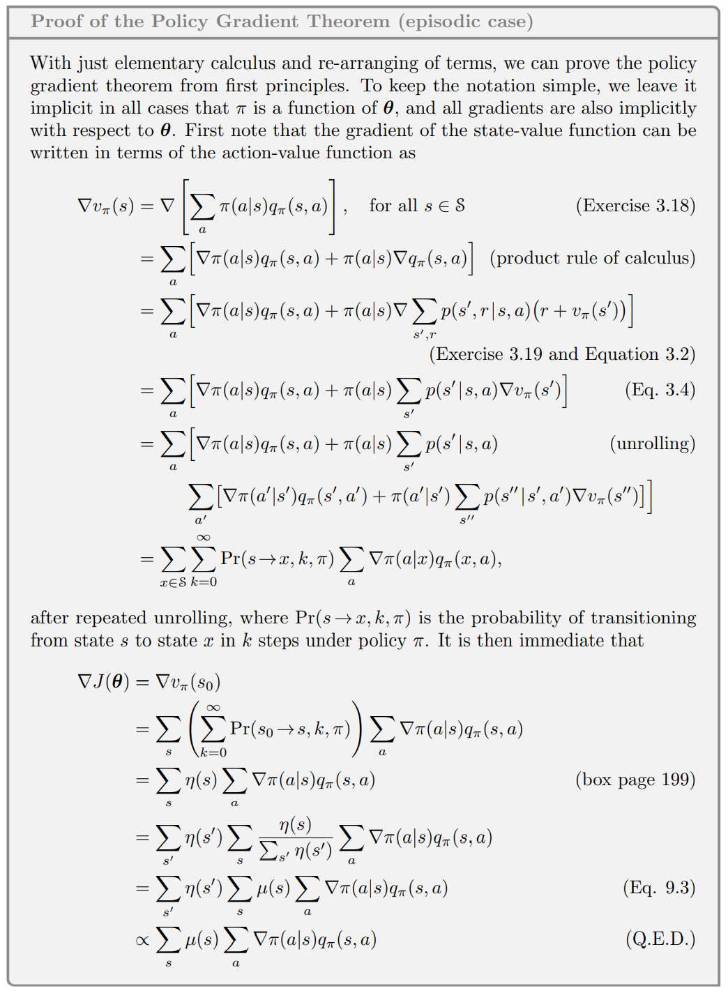
The proof of this is what the Policy Gradient Theorem is all about. The derivation is a lot of fun.

2.1.1 The Policy Gradient Theorem (episodic case)

Figure 1

Under construction $$\begin{aligned}$$

An optional caption for a math block

2.1.2 Monte Carlo Policy Gradient Algorithm

Under construction